

Python: from data to your own digest Lesson 29 of 56
Grouping and aggregates: counting by category and by month
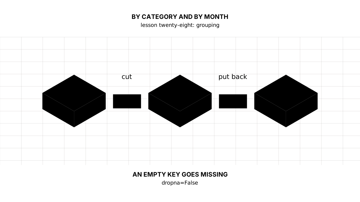
The twenty-eighth lesson of the Python course. `groupby` is a loop written as a question: cut the table by a key, count each piece, put the pieces back. `agg` with column names of your own, two keys, a key the table does not hold, `transform` for a share, the difference between `count` and `size`, and the groups that go missing without a word.
Why this matters
The last lesson kept the rows that mattered. This one answers the question they are usually kept for: how much per category, per city, per month.
As a loop it goes: an empty dictionary, a walk over the rows, an accumulation, then a second walk to work out the averages. We have written that loop more than once — in lesson six it was the subject. groupby does the same in one line, and what matters about it is not the brevity but that the question is visible whole: what we group by, and what we count.
If you remember GROUP BY from lesson twenty-two — this is that, over a table in your own program’s memory.
The whole thing first
The file is gruppy.py. Twelve receipts over two months and seven ways to add them up.
"""Lesson 28: grouping and aggregates.

Twelve receipts over two months. Counted by category, by city and by month --
and not a loop in sight.
"""

import pandas as pd

rows = [
    ("2026-01-03", "Kostanay", "food", 4200),
    ("2026-01-05", "Kostanay", "fuel", 18500),
    ("2026-01-07", "Rudny", "food", 2600),
    ("2026-01-09", "Kostanay", "phone", 4990),
    ("2026-01-15", "Kostanay", "rent", 95000),
    ("2026-01-18", "Rudny", "fuel", 16200),
    ("2026-01-24", "Kostanay", "food", 3100),
    ("2026-02-02", "Rudny", "food", 2800),
    ("2026-02-06", "Kostanay", "fuel", 19100),
    ("2026-02-11", "Kostanay", "phone", 4990),
    ("2026-02-15", "Kostanay", "rent", 95000),
    ("2026-02-20", "Rudny", "rent", 62000),
]
df = pd.DataFrame(rows, columns=["day", "city", "kind", "amount"])
df["day"] = pd.to_datetime(df["day"])

print("== the sum per category")
print(df.groupby("kind")["amount"].sum().sort_values(ascending=False))

print()
print("== three numbers at once")
print(df.groupby("kind")["amount"].agg(["count", "sum", "mean"]).round(0))

print()
print("== column names of your own")
report = df.groupby("kind").agg(
    receipts=("amount", "count"),
    total=("amount", "sum"),
    average=("amount", "mean"),
).round(0)
print(report.sort_values("total", ascending=False))

print()
print("== two keys")
by_two = df.groupby(["city", "kind"])["amount"].sum()
print(by_two)
print("labels:", type(by_two.index).__name__)

print()
print("== back to a flat table")
print(by_two.reset_index().head(3))

print()
print("== by month: a key the table does not hold")
by_month = df.groupby(df["day"].dt.to_period("M"))["amount"].agg(["count", "sum"])
print(by_month)

print()
print("== count counts values that are there, size counts rows")
with_gap = df.copy()
with_gap.loc[6, "amount"] = None
print("count:", with_gap.groupby("kind")["amount"].count().to_dict())
print("size: ", with_gap.groupby("kind").size().to_dict())

print()
print("== the share of a category inside its city")
df["share"] = (df["amount"] / df.groupby("city")["amount"].transform("sum") * 100).round(1)
print(df.loc[df["city"] == "Rudny", ["kind", "amount", "share"]].to_string(index=False))
It prints:
== the sum per category
kind
rent     252000
fuel      53800
food      12700
phone      9980
Name: amount, dtype: int64

== three numbers at once
       count     sum     mean
kind
food       4   12700   3175.0
fuel       3   53800  17933.0
phone      2    9980   4990.0
rent       3  252000  84000.0

== column names of your own
       receipts   total  average
kind
rent          3  252000  84000.0
fuel          3   53800  17933.0
food          4   12700   3175.0
phone         2    9980   4990.0

== two keys
city      kind
Kostanay  food       7300
          fuel      37600
          phone      9980
          rent     190000
Rudny     food       5400
          fuel      16200
          rent      62000
Name: amount, dtype: int64
labels: MultiIndex

== back to a flat table
       city   kind  amount
0  Kostanay   food    7300
1  Kostanay   fuel   37600
2  Kostanay  phone    9980

== by month: a key the table does not hold
         count     sum
day
2026-01      7  144590
2026-02      5  183890

== count counts values that are there, size counts rows
count: {'food': 3, 'fuel': 3, 'phone': 2, 'rent': 3}
size:  {'food': 4, 'fuel': 3, 'phone': 2, 'rent': 3}

== the share of a category inside its city
kind  amount  share
food    2600    3.1
fuel   16200   19.4
food    2800    3.3
rent   62000   74.2
Going through it
Cut, count, put back
df.groupby("kind")["amount"].sum() does three things: it cuts the table into pieces by the value of kind, counts the sum in each, and puts the pieces back together as one series. The key becomes a label — the very index from lesson twenty-five — so the answer can be sorted, filtered and added to another series like it straight away.
The default order of the groups is by the key, ascending, not by the size of the answer. A ranking is asked for separately: .sort_values(ascending=False).
Several numbers at once, and names of your own
agg(["count", "sum", "mean"]) gives three columns instead of one. Their names are the names of the functions, and in a report they look like a draft.
The named form reads like the definition of the report:
df.groupby("kind").agg(
    receipts=("amount", "count"),
    total=("amount", "sum"),
    average=("amount", "mean"),
)
On the left, the name of the column in the answer; on the right, the pair (column, aggregation function): which column to count and what to count it with. One agg can mix different columns: dearest=("amount", "max"), first_day=("day", "min").
count counts the values that are there, size counts all the rows
The difference is not cosmetic. count counts the values a column holds — any of them: numbers, strings, dates — and passes over the missing ones. size counts the rows of the group whole. The gap between them is exactly the number of missing values in the column you counted. In the example, after one value was erased, count says 3 for food and size says 4.
Hence the difference in how they are asked: count is asked of a column (groupby(...)["amount"].count()), size of the group itself, which needs no column.
That is the first of two ways to get a wrong answer in silence. The second is worse.
The groups that go missing
By default groupby throws away the rows whose key is empty. The sum over the groups then does not match the sum over the table, and nothing says so:
df["amount"].sum()                        → 1000
df.groupby("kind")["amount"].sum().sum()  → 800
The cure is the argument dropna=False: the gap becomes a group of its own. A habit worth acquiring: after a grouping, check the total against the total over the whole table. If they differ, you already know where to look.
Two keys and labels in two storeys
groupby(["city", "kind"]) gives a MultiIndex: the row’s label is a pair. That is convenient to look at and inconvenient to pass on, so most of the time .reset_index() follows immediately — and gives an ordinary flat table with the two keys as columns.
A key the table does not hold
You can group not only by a column but by any series of the same length. Hence “by month”: df["day"].dt.to_period("M") turns a date into a month, and that is what we group by — there need be no “month” column in the table at all.
to_period("M") gives a period rather than the string "2026-01": it sorts as time rather than as text, and it can have a number of months added to it. For days there is dt.date, for years dt.year, for weekdays dt.day_name().
transform: the group’s answer beside every row
agg squeezes a group into one number. transform gives back as many values as there were rows — the same group number, repeated across the rows of its own group. Hence the share:
df["amount"] / df.groupby("city")["amount"].transform("sum") * 100
Every row has the sum of its own city in the denominator. The same move gives the deviation from a group average and the rank within a group (rank).
The map of this lesson
Say it in your own words
Without looking, answer out loud or on paper. The answers are at the end of the lesson.
- What does
groupbydo, and what does the key become in the answer? - How does
countdiffer fromsize, and what does the difference between them mean? - How does
transformdiffer fromagg, and when is it the one you want?
The warm-up
Three short steps before the exercise: predict, fill in, fix. The answers are at the end, but answer for yourself first.
1. Predict. What does this program print?
import pandas as pd

df = pd.DataFrame({"kind": ["food", "food", "phone"], "amount": [1200, 800, 4990]})
print(df.groupby("kind")["amount"].sum().to_dict())
print(df.groupby("kind")["amount"].agg(["count", "max"]).to_string())
2. Fill in the blank. In place of ... name the column “total” and count the sum in it.
# a named aggregate: the name on the left, the pair "column, what with" on the right
import pandas as pd

df = pd.DataFrame({"kind": ["food", "food", "phone"], "amount": [1200, 800, 4990]})
print(df.groupby("kind").agg(...).to_string())
3. Fix it. The sum over the groups falls two hundred short of the sum over the table. Nothing was lost — one group simply never made it into the answer.
# 1000 against 800: where the other two hundred went
import pandas as pd

df = pd.DataFrame({"kind": ["food", None, "food", "phone"], "amount": [100, 200, 300, 400]})
print("in total:", int(df["amount"].sum()))
print("by group:", int(df.groupby("kind")["amount"].sum().sum()))
The exercise
Required. Take the same twelve receipts from the lesson and build a report by month and category: the number of receipts, the sum, and the share of the category inside its own month. Sort the report by month, and inside a month by sum from the top down. At the end print the totals per month and the month that cost more.
The expected output:
  month  kind  receipts  total  share
2026-01  rent         1  95000   65.7
2026-01  fuel         2  34700   24.0
2026-01  food         3   9900    6.8
2026-01 phone         1   4990    3.5
2026-02  rent         2 157000   85.4
2026-02  fuel         1  19100   10.4
2026-02 phone         1   4990    2.7
2026-02  food         1   2800    1.5

the totals per month: {'2026-01': 144590, '2026-02': 183890}
the month that cost most: 2026-02
Done when: the output matches line for line; the share is computed against the sum of its own month rather than of both; the columns are named in agg rather than renamed afterwards; the month comes out of the date rather than being cut out of a string; the costliest month is found with idxmax.
On your own data. Group a table of yours by any field and compute three numbers. Then check: does the sum over the groups equal the sum over the whole table? If it does not, look for gaps in the key.
If you feel like it.
- Group by weekday (
dt.day_name()) and see which day costs more. - Add a column from another field to the
agg:first_day=("day", "min"). - Use
transform("mean")to compute each receipt’s deviation from the average of its category.
Where this fits the project
Step nine: the digest stops watching one country. Three of them arrive in a single request — the bank takes the codes separated by semicolons — and the table becomes long: one row per country and year.
That shape is what it was all for: the report turns into one question instead of a loop over countries. groupby("country").agg(...) gives the years, the gaps, the average and the maximum, and the year of the maximum comes from idxmax inside the grouping — the label of the largest value is that row, and the row knows its year.
Still open. The countries in the report are called KAZ, UZB, RUS, because that is how the bank hands them over. Their names are in the same answer, but putting them alongside needs a second table and a join on a key. That is the next lesson.
The answers
To the questions
- It cuts the table into pieces by the key, counts each piece separately and puts the answers back together as a table. The key becomes the row’s label — the index — so the answer can be sorted and added to other series by those same labels.
countcounts the values that are there — numbers, strings, dates, anything;sizecounts every row of the group. Their difference is the number of gaps in the column you counted.aggsqueezes a group into one number;transformreturns as many values as there are rows, repeating the group’s number for every row of its own group. It is what you want when a group’s answer has to stand beside the original rows: a share, a deviation from the average, a rank within the group.
To the warm-up
- Grouping by category gives the sum of each, and
aggwith a list gives two columns named after the functions.
{'food': 2000, 'phone': 4990}
       count   max
kind
food       2  1200
phone      1  4990
total=("amount", "sum"). The column’s name on the left of the equals sign, the pair “what to count, what with” on the right.
import pandas as pd

df = pd.DataFrame({"kind": ["food", "food", "phone"], "amount": [1200, 800, 4990]})
print(df.groupby("kind").agg(total=("amount", "sum")).to_string())
       total
kind
food    2000
phone   4990
groupby("kind", dropna=False). A row whose key is empty falls into no group by default, and two hundred leave without a word.
import pandas as pd

df = pd.DataFrame({"kind": ["food", None, "food", "phone"], "amount": [100, 200, 300, 400]})
print("in total:", int(df["amount"].sum()))
print("by group:", int(df.groupby("kind", dropna=False)["amount"].sum().sum()))
in total: 1000
by group: 1000
To the exercise
The share is computed with transform("sum") over the month: every row needs the sum of its own month in the denominator, not the overall one. Divide by report["total"].sum() and the shares add up to a hundred per cent across the whole report rather than within each month — a different answer to a different question.
The sorting takes two keys at once: sort_values(["month", "total"], ascending=[True, False]), because the months go in order while the sums inside a month go from larger to smaller.
Sources
- Group by: split-apply-combine — how it works and what else it can do.
- Named aggregation — the form in which a report reads as a report.
- Time series and date functionality —
dt, periods and everything time can be grouped by.
If you have found a mistake or a typo in this article, tell us about it
Comments (0)
Log in to leave a comment →
No comments yet. Be the first.