

Python: from data to your own digest Lesson 45 of 56
Training and checking: why a model cannot mark its own work
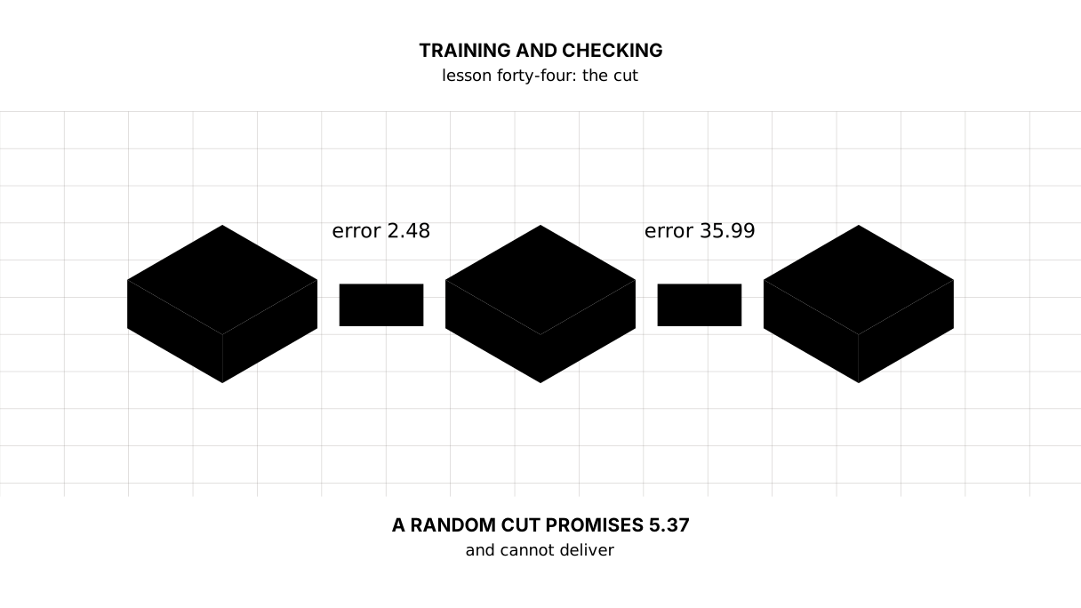
The forty-fourth lesson of the Python course. The same model on the same data: an error of 2.48 points on the years it was taught, and 35.99 on the years it never saw. A random cut instead of a cut by time shows 5.37 and lies. A fifth-degree polynomial learns almost perfectly and is three times worse than a line.
Why this matters
The last lesson ended with an admission: both models were measured on the very years they learned from. That is how everything marks itself — and it is the one check a model always passes.
An honest check costs one line of code and changes every conclusion. This lesson is about cutting a series by time, why a random cut lies here, and what overfitting looks like once it can be seen at all.
The whole thing first
The file is proverka.py. The series is the one from the last lesson: the consumer price index of Kazakhstan, from the World Bank.
"""Lesson 44: training and checking -- why a model cannot mark its own work.

The series is the one from the last lesson: the consumer price index of
Kazakhstan, 2010 = 100, the World Bank indicator FP.CPI.TOTL.
"""

import numpy as np
import pandas as pd
from sklearn.linear_model import LinearRegression
from sklearn.metrics import mean_absolute_error
from sklearn.model_selection import train_test_split

CPI = pd.Series({
    2010: 100.00, 2011: 108.45, 2012: 114.09, 2013: 120.87, 2014: 129.15,
    2015: 137.77, 2016: 157.56, 2017: 169.28, 2018: 179.72, 2019: 189.30,
    2020: 202.02, 2021: 218.27, 2022: 251.07, 2023: 287.54, 2024: 312.53,
    2025: 348.12,
})
YEARS = CPI.index.to_numpy()
VALUES = CPI.to_numpy()

# The years are moved to zero and divided by ten: large numbers raised to a
# power are counted badly, and powers are needed below.
def feature(years, degree=1):
    return np.vander((years - 2010) / 10, degree + 1)


def log_line(years, values):
    """The line through the logarithm -- the shape from the last lesson."""
    model = LinearRegression().fit(feature(years), np.log(values))
    return lambda ask: np.exp(model.predict(feature(ask)))


print("== The cut by time")
past = YEARS <= 2021
guess = log_line(YEARS[past], VALUES[past])
on_train = mean_absolute_error(VALUES[past], guess(YEARS[past]))
on_test = mean_absolute_error(VALUES[~past], guess(YEARS[~past]))
print("  trained on:", int(YEARS[past].min()), "-", int(YEARS[past].max()),
      f"({int(past.sum())} years)")
print("  checked on:", [int(y) for y in YEARS[~past]])
print("  the error on training:", round(on_train, 2), "points")
print("  the error on the check:", round(on_test, 2), "points")
print("  the check is worse by a factor of", round(on_test / on_train, 1))

print()
print("== A random cut flatters")
y_train, y_test, v_train, v_test = train_test_split(
    YEARS, VALUES, test_size=4, random_state=0)
shuffled = log_line(y_train, v_train)
print("  the check years:", [int(y) for y in sorted(y_test)])
print("  the error on the check:", round(mean_absolute_error(v_test, shuffled(y_test)), 2), "points")
print("  the same model on the cut by time:", round(on_test, 2), "points")

print()
print("== The more complex, the worse")
rows = []
for degree in (1, 2, 3, 5):
    model = LinearRegression().fit(feature(YEARS[past], degree), VALUES[past])
    rows.append({
        "degree": degree,
        "on training": round(mean_absolute_error(
            VALUES[past], model.predict(feature(YEARS[past], degree))), 2),
        "on the check": round(mean_absolute_error(
            VALUES[~past], model.predict(feature(YEARS[~past], degree))), 2),
    })
table = pd.DataFrame(rows).set_index("degree")
print(table.to_string())

print()
print("== What to choose")
best_train = table["on training"].idxmin()
best_test = table["on the check"].idxmin()
print("  best degree by training:", best_train, "— on the check it gives",
      table.loc[best_train, "on the check"])
print("  best degree by the check:", best_test, "— on the check it gives",
      table.loc[best_test, "on the check"])
print("  the line in logarithms:", round(on_test, 2), "— better than every polynomial")
The output:
== The cut by time
  trained on: 2010 - 2021 (12 years)
  checked on: [2022, 2023, 2024, 2025]
  the error on training: 2.48 points
  the error on the check: 35.99 points
  the check is worse by a factor of 14.5

== A random cut flatters
  the check years: [2011, 2016, 2018, 2019]
  the error on the check: 5.37 points
  the same model on the cut by time: 35.99 points

== The more complex, the worse
        on training  on the check
degree
1              3.51         60.78
2              2.30         41.22
3              2.13         57.09
5              0.99        116.69

== What to choose
  best degree by training: 5 — on the check it gives 116.69
  best degree by the check: 2 — on the check it gives 41.22
  the line in logarithms: 35.99 — better than every polynomial
The walk-through
The check is the years the model never saw
  the error on training: 2.48 points
  the error on the check: 35.99 points
The model and the data are the same as in lesson forty-three. One thing changed: it was taught on 2010–2021 and asked about 2022–2025. The error grew by a factor of 14.5.
Neither number is the “real” one with the other a fake. They simply answer different questions. The training error says how well the model described the past; the check error says how far it will do for what such a model is usually built for.
A random cut flatters, and here is why
  the check years: [2011, 2016, 2018, 2019]
  the error on the check: 5.37 points
  the same model on the cut by time: 35.99 points
train_test_split shuffles the data — by default, and without asking. On a table of customers that is right. On a series over time it is a forgery: 2019 becomes a check year while 2018 and 2020 stay in the training, and the model does not predict 2019, it inserts it between two known points. The problem “what comes next” turns into “what was in the middle”, which is incomparably easier.
Worse, with a random cut the model sees the future: years that come after the check years end up in the training. In real work that never happens, and the figure 5.37 is a promise the model will not keep even once.
The rule: a series over time is cut by time. The last years are the check, and only they.
Overfitting is visible only when there is a check
        on training  on the check
1              3.51         60.78
2              2.30         41.22
3              2.13         57.09
5              0.99        116.69
The fifth-degree polynomial describes the past almost perfectly — an error of less than a point. On the years it did not see it is off by 117 points: it learned not the shape of the series but its particulars, down to the accidental ones.
That is overfitting, and notice: the left column does not show it. There everything looks like an improvement. Overfitting is not a property of a model you can inspect; it is the difference between two columns.
Choose on validation and leave the test until the end
  best degree by training: 5 — on the check it gives 116.69
  best degree by the check: 2 — on the check it gives 41.22
If a model is chosen by how it described the past, the choice falls on the worst one available. The task counts the difference as a number: 75 points is the price of one wrong criterion.
And separately: the line in logarithms, the one with the right shape, gives 35.99 on the check and beats every polynomial. Shape matters more than complexity — the same conclusion as the last lesson, only now it is drawn on data the model never saw.
What this count cannot do
There are four check years. That is better than none and still few: had a quiet year fallen among them instead of 2022, the numbers would be different. The honest conclusion from a check like this is “the model is off by tens of points”, not “the model is off by 35.99”.
In this teaching example the last four years are validation data used to compare model forms. No independent test remains after that choice, so these errors are not a final estimate of performance. In real work, reserve a later test period and inspect it once after model selection.
And one more thing to keep from this lesson: validation years are spent. Pick a model by looking at the check, do that ten times, and the check slowly turns into training — just by a slower route.
The lesson map
Say it in your own words
Answer out loud or on paper without looking. The answers are at the end of the lesson.
- Why is the training error almost always smaller than the check error?
- What is wrong with a random cut on a series over time?
- What does overfitting look like in two columns of errors?
Warm-up
Three short steps before the task: predict, fill in, fix. The answers are at the end of the lesson, but answer for yourself first.
1. Predict. Which years end up in the check, and will they run consecutively?
import numpy as np
from sklearn.model_selection import train_test_split

years = np.arange(2010, 2026)
train, test = train_test_split(years, test_size=4, random_state=0)
print("check years:", [int(y) for y in sorted(test)])
print("do they run consecutively:", sorted(int(y) for y in test) == list(range(2022, 2026)))
2. Fill in the blank. In place of ... separate the last four years with no randomness at all.
# the last four years go to the check, the rest to the training
import numpy as np

years = np.arange(2010, 2026)
past = ...
print("training:", int(years[past].min()), "-", int(years[past].max()))
print("the check:", [int(y) for y in years[~past]])
3. Fix it. The program prints one error and calls it the quality of the model.
# the quality of a model is two errors, not one
import numpy as np
from sklearn.linear_model import LinearRegression
from sklearn.metrics import mean_absolute_error

years = np.arange(2010, 2026).reshape(-1, 1)
values = np.array([100.0, 108.45, 114.09, 120.87, 129.15, 137.77, 157.56, 169.28,
                   179.72, 189.3, 202.02, 218.27, 251.07, 287.54, 312.53, 348.12])
model = LinearRegression().fit(years, values)
print("the error:", round(mean_absolute_error(values, model.predict(years)), 2))
The task
Required. Cut the series by time: the last four years are the check. Print what is in each part, and on a line of its own make sure no year ended up in both. Train the line in logarithms, print both errors and how many times worse the check is. Then walk the degrees of a polynomial from one to five and print a table of both errors; name the degree chosen by the training, the degree chosen by the check, and the price of the wrong choice in points. At the end repeat the cut at random with three different seeds and show those errors next to the honest one.
The expected output:
== The cut by time
  training: [2010, 2011, 2012, 2013, 2014, 2015, 2016, 2017, 2018, 2019, 2020, 2021]
  the check: [2022, 2023, 2024, 2025]
  years in both parts: none
  the line in logarithms: training 2.48 — check 35.99
  the check is worse by a factor of 14.5

== The degrees of a polynomial
        on training  on the check
degree
1              3.51         60.78
2              2.30         41.22
3              2.13         57.09
4              2.13         52.01
5              0.99        116.69
  chosen by training: 5 — on the check it gives 116.69
  chosen by the check: 2 — on the check it gives 41.22
  the price of the wrong choice: 75.47 points

== A random cut, three tries
  seed 0: check years [2011, 2016, 2018, 2019] — error 5.37
  seed 1: check years [2012, 2013, 2017, 2023] — error 4.54
  seed 42: check years [2010, 2011, 2015, 2024] — error 7.68
  by time: 35.99 — and that is the only honest figure
Done means: the output matches line for line; the leak check is printed always rather than only when there is a leak; the degree is chosen by the code for each of the two criteria separately; the random cuts are made with seeds written down, or the numbers will not come back.
On your own data. Take a series of your own over time and cut off the last fifth. Train anything — even a mean — on the first part and look at the error on the second. It almost always turns out noticeably bigger than what you saw before, and that is fine: you have just measured for the first time what you meant to measure.
If you want more.
- Move the boundary of the cut to 2019 and see how both errors change: the check gets longer and 2022 falls into it.
- Check the model with a rolling window: train on the years up to N, ask about N + 1, and so on for every N. That gives a series of errors instead of one number.
- See what
train_test_split(..., shuffle=False)does: the cut becomes sequential, which is the closest thing to honest among the ready-made options.
Where this goes in the project
Step twenty-three: the digest asks its model about a year it did not see.
esep.trend now teaches the line a second time — without the last year — and asks about it. Both errors stand on the page: Kazakhstan is off by 3.55 on its own years and 4.85 on the held-out one, Uzbekistan by 1.02 and 2.56. For Russia it is the other way round: 2.95 and 1.32, more accurate on the year it never saw. That happens when the check has a single point, and it is exactly why the column is not called “the real error”: one held-out year is the beginning of a check, not a verdict.
There is still no forecast. A line that misses a known year by five points does not become trustworthy about an unknown one because it was asked politely.
The same step fixes the store. saqtau.save wrote the rates with two decimals, and one and the same report said 3.55 on a run that went to the network and 3.56 on a run that read the file. Two decimals are enough for a rate of inflation and not enough for a line fitted through sixteen of them. A store that changes the answer is not a store.
The answers
To the questions
- Because in training the model fitted its coefficients to those very points — it saw the answers. On the check it answers for the first time. A gap of one and a half to two times is ordinary; a gap of fourteen, as here, means the model described the past rather than a regularity.
- Because shuffling puts a check year between known ones, and the problem “predict” is swapped for the problem “fill in the missing”. On top of that, years that in reality come after the check years end up in the training — the model sees the future. The figure comes out pretty and impossible.
- The left column falls, the right one grows. On its own the left column says nothing about overfitting: for the fifth degree it is the best of all, and on the check that model is the worst.
To the warm-up
train_test_splitshuffles by default, so the years are scattered across the series and do not run consecutively.
check years: [2011, 2016, 2018, 2019]
do they run consecutively: False
years <= 2021. A comparison with a year rather than randomness: the boundary of the cut is visible in the code and does not change from run to run.
# the last four years go to the check, the rest to the training
import numpy as np

years = np.arange(2010, 2026)
past = years <= 2021
print("training:", int(years[past].min()), "-", int(years[past].max()))
print("the check:", [int(y) for y in years[~past]])
training: 2010 - 2021
the check: [2022, 2023, 2024, 2025]
- The model learned on the whole series, so the error printed is the training error. The series has to be cut and both printed.
# the error is measured on years the model did not see
import numpy as np
from sklearn.linear_model import LinearRegression
from sklearn.metrics import mean_absolute_error

years = np.arange(2010, 2026).reshape(-1, 1)
values = np.array([100.0, 108.45, 114.09, 120.87, 129.15, 137.77, 157.56, 169.28,
                   179.72, 189.3, 202.02, 218.27, 251.07, 287.54, 312.53, 348.12])
past = (years <= 2021).ravel()
model = LinearRegression().fit(years[past], values[past])
print("on training:", round(mean_absolute_error(values[past], model.predict(years[past])), 2))
print("on the check:", round(mean_absolute_error(values[~past], model.predict(years[~past])), 2))
on training: 3.51
on the check: 60.78
To the task
The line about the leak is printed every time, and that is not a formality. A leak rarely looks like an error: the code runs, the numbers come out pretty, and the only sign is that they are too pretty. A check that prints “none” every time costs little and finds what is otherwise not found at all.
Three random cuts give 5.37, 4.54 and 7.68 — all of them several times smaller than the honest 35.99. Notice that they do not agree with each other either: the seed decides not only how pretty the figure is but what the figure is. When a result depends on a random number, it is printed together with that number.
Sources
- train_test_split, scikit-learn — the
shuffleandrandom_stateparameters that cause all of this. - Cross-validation of time series, scikit-learn —
TimeSeriesSplit, a ready-made cut by time. - Consumer price index, World Bank — the series the lesson is built on.
If you have found a mistake or a typo in this article, tell us about it
Comments (0)
Log in to leave a comment →
No comments yet. Be the first.